

Welcome to Lesson 3 in our Python SDK learning series. Each lesson is independent, but make sure you check out Lesson 1 and Lesson 2.
This lesson is about creating your own polygons and leveraging Oceanbolt’s algorithms to do vessel counts – quickly at scale. You can follow along in this Jupyter Notebook or read the summary below.
Oceanbolt Python SDK Lesson 3: Custom Polygons
At Oceanbolt, a core part of our work is geospatial analytics. We use geofences (or polygons as we refer to them internally) to build our cargo tracking algorithms and to infer what the dry bulk fleet is doing (now and historically). While we provide our users with a fully mapped world of dry bulk infrastructure (e.g. ports, berths, terminals), a user may have a desire to create her or his own polygons to monitor particular areas of interest. An example of this may be a Handysize operator, who thinks differently about zones, than a Capesize operator does.
We have therefore introduced the functionality to unleash the power of Oceanbolt’s algorithms on a user’s “self-defined” or “custom” polygons. All that is required are the coordinates that make up the user-defined polygons.
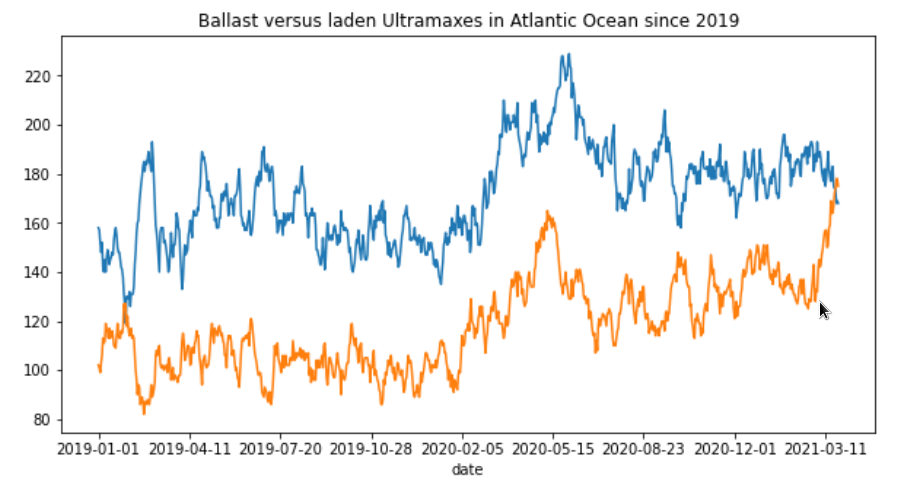
In the example below, we create a polygon of the Atlantic Ocean to track the number of Ultramaxes in laden and ballast status since 2019. The calculation on this polygon to get all historical daily counts since 2019 takes less than 1 second (pretty fast, yes!).
How to generate polygons
In order to generate counts, we need a polygon and its coordinate in GeoJSON format. There are many tools available to create and manage polygons and geospatial layers, e.g. QGIS and geojson.io. For our purpose, we use geojson.io, as it is quick and easy to use and directly prints the coordinates for the polygons required GeoJSON string.
Below you will find a GIF outlining how we get the polygon coordinates for the Atlantic Ocean by using geojson.io.
NOTE: The polygon is rather crude and users may actually be more diligent in properly drawing the polygons.
Now that we have the polygon ready, we turn to the Oceanbolt Python SDK to write the actual script. Here is a sample of the code from the Jupyter Notebook. You can follow along in the notebook to get a better understanding of the steps.
from oceanbolt.sdk.client import APIClient
    from oceanbolt.sdk.data.tonnage import CustomPolygonTimeseries
    from datetime import date
    import time

    # Counting the number of laden Ultramaxes in our Polygon
    df_ultra_laden = CustomPolygonTimeseries(base_client).get(
    geom_polygon="{\"type\":\"Polygon\",\"coordinates\":[[[-48.515625,61.10078883158897],[-81.5625,29.53522956294847],[-66.796875,13.239945499286312],[-50.2734375,1.0546279422758869],[-33.046875,-5.615985819155327],[-53.0859375,-34.88593094075315],[-70.3125,-50.736455137010644],[-64.6875,-56.170022982932046],[-25.3125,-56.94497418085159],[18.984375,-46.07323062540835],[18.984375,-29.22889003019423],[9.4921875,4.214943141390651],[-13.0078125,5.61598581915534],[-17.2265625,20.3034175184893],[-7.734374999999999,35.17380831799959],[-12.3046875,50.28933925329178],[-14.765625,62.75472592723178],[-48.515625,61.10078883158897]]]}",
    #Polygon coordinates corresponding to polygon that we drew.
    sub_segment=['ultramax'],
    laden_status=['laden'],
    start_date=date(2019,1,1),
    end_date=date(2021,3,25),
    )

    # Counting the number of ballasting Ultramaxes in our Polygon
    df_ultra_ballast = CustomPolygonTimeseries(base_client).get(
    geom_polygon="{\"type\":\"Polygon\",\"coordinates\":[[[-48.515625,61.10078883158897],[-81.5625,29.53522956294847],[-66.796875,13.239945499286312],[-50.2734375,1.0546279422758869],[-33.046875,-5.615985819155327],[-53.0859375,-34.88593094075315],[-70.3125,-50.736455137010644],[-64.6875,-56.170022982932046],[-25.3125,-56.94497418085159],[18.984375,-46.07323062540835],[18.984375,-29.22889003019423],[9.4921875,4.214943141390651],[-13.0078125,5.61598581915534],[-17.2265625,20.3034175184893],[-7.734374999999999,35.17380831799959],[-12.3046875,50.28933925329178],[-14.765625,62.75472592723178],[-48.515625,61.10078883158897]]]}",
    sub_segment=['ultramax'],
    laden_status=['ballast'],
    start_date=date(2019,1,1),
    end_date=date(2021,3,25),
    )
In the Jupyter Notebook you will see an additional code snippet that calculates the time it takes to run each of these operations. As per the notebook, it takes 0.7 seconds to get the laden vessels and 0.5 seconds to get the ballast vessels. Note that this includes all historical counts going back to 01 Jan 2019 up until today.
We continue to plot the timeseries:
df_ultra_laden['ballast'] = df_ultra_ballast['value']
    df_ultra_laden.plot(x='date', y=['value', 'ballast'], figsize=(10,5), title='Ballast versus laden Ultramaxes in Atlantic Ocean since 2019', legend=False);
The resulting output, we get is the chart below with ballaster in orange and laden in blue.
Thanks for reading this! If you are interested in getting access to our data, sign up for a product demo and stay tuned for future lessons!
NOTE: The custom polygons feature will be available in our web-based dashboard to allow non-Python users to define their own polygons as well.