Oceanbolt Python SDK Lesson 1 – Fleet Utilization

Last week we introduced our Python SDK, which allows our users to programmatically interact with our data in an automated, friction-less manner.

Our Python SDK is richly documented and includes sample Python Notebooks on GitHub illustrating how to use the SDK for, among other things, finding iron Ore imports by Capes in China or listing port calls in Santos.

While the sample notebooks are helpful, we recognize the examples only illustrate the top of iceberg of what is possible with our Python SDK. Therefore, we have decided to do a couple of blog post that go a bit deeper on certain topics that are central to the Oceanbolt community of maritime professionals, commodity traders, market intelligence/business developers and financial analysts.

In this first lesson is about fleet utilization and its different methodologies. You can follow along in this Jupyter Notebook or read the summary below.

Oceanbolt Python SDK Lesson 1: Fleet Utilization

One of the central questions to anyone in the dry bulk shipping space is “What is the current utilization of the fleet in my market?”. An iron ore focused shipping professional might ask this question for the Capesize fleet, while a copper concentrate focused shipping professional might think about utilization for the Handysize & Supramax fleet. In this Oceanbolt Python SDK lesson, we will focus on utilization for the Panamax fleet – a vessel segment heavily involved in coal and grains freight.

In order to determine fleet utilization, it is helpful to clarify that there are several methodologies for determining fleet utilization. In this article, we will look at two popular fleet utilization methodologies:

1. Tonnage Demand/Supply: Demand as measured in volume, ton-miles, or ton-days versus total available fleet capacity

2. Employed vessels: Number of vessels in ballast at sea versus total number of vessels active

Each of these methodologies have strengths and drawbacks. The first methodology is (in our opinion) the most widespread among shipping professionals. It has a clear economic rationale as it is based on demand for freight (as measured in volume, ton-miles or ton-days) and supply measured in available vessel capacity. A big drawback of this methodology, however, is that determining “available vessel capacity” will inevitably force us to introduce additional assumptions (which may or may not be backed by data) to be able to match the units of demand and supply in order to calculate the utilization. You can check the Jupyter Notebook to see how this plays out for our calculations. The biggest drawback, however, is that we do not get a daily timeseries from this methodology, so appyling statistics and machine learning is not feasible.

The other methodology, the “employed vessels” methodology, is simpler. While crude in its economic rationale, it offers the advantages of being simple to calculate, easy to understand, and most importantly offers the ability to create a daily timeseries without making any additional assumptions.

The “employed vessels” methodology simply counts the total number of vessels ballasting at sea (making a crude assumption that these vessels are not employed) and measures this tonnage as the available tonnage. Utilization thus becomes employed tonnage divided by total tonnage.

Here is a sample of the code from the Jupyter Notebook.

from oceanbolt.sdk.client import APIClient
    from oceanbolt.sdk.data.tonnage import TonnageZoneTimeseries
    from oceanbolt.sdk.data.trade_flows import TradeFlowTimeseries
    from datetime import date
    import pandas as pd
   
   df1 = tonnage_zone_client.get(
    sub_segment=['panamax'], #We select the vessel sub-segment of Panamaxes in DWT68k-80k. A list of all available segments can be achieved by calling our Segments Entities API (https://python-sdk.oceanbolt.com/entities_v3/segments.html).
    start_date=date(2020, 1, 1), 
    end_date=date(2020, 12, 31),  
    )
   
   df2 = tonnage_zone_client.get(
    sub_segment=['panamax'], # We select Panamax vessels
    laden_status=["ballast"], # We select Panamax vessels that are ballasting
    port_status=["at_sea"], # We select Panamax vessels that are ballasting at sea
    start_date=date(2020, 1, 1), 
    end_date=date(2020, 12, 31),  
    )
    
    df3 = pd.DataFrame(1-df2['vessel_dwt']/df1['vessel_dwt'])
    df3['date'] = df1['date']
    df3.plot(x='date', figsize=(10,5), title='Oceanbolt 2020 Panamax Fleet Utilzation', legend=False)

By using the employed vessels methodology, we obtain the following chart.

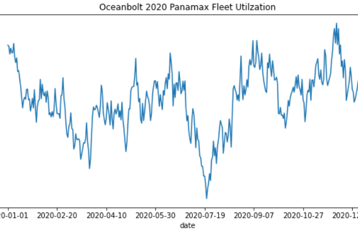
It becomes clear that from the two methodologies, “employed vessels” works without making outrageous assumptions and gives a daily timeseries. A daily timeseries would have allowed us to use statistics or machine learning to infer whether there is a relationship between freight rates and utilization. We will leave this for another lesson.

Thanks for reading this! If you are interested in getting access to our data, sign up for a product demo and stay tuned for future lessons!